
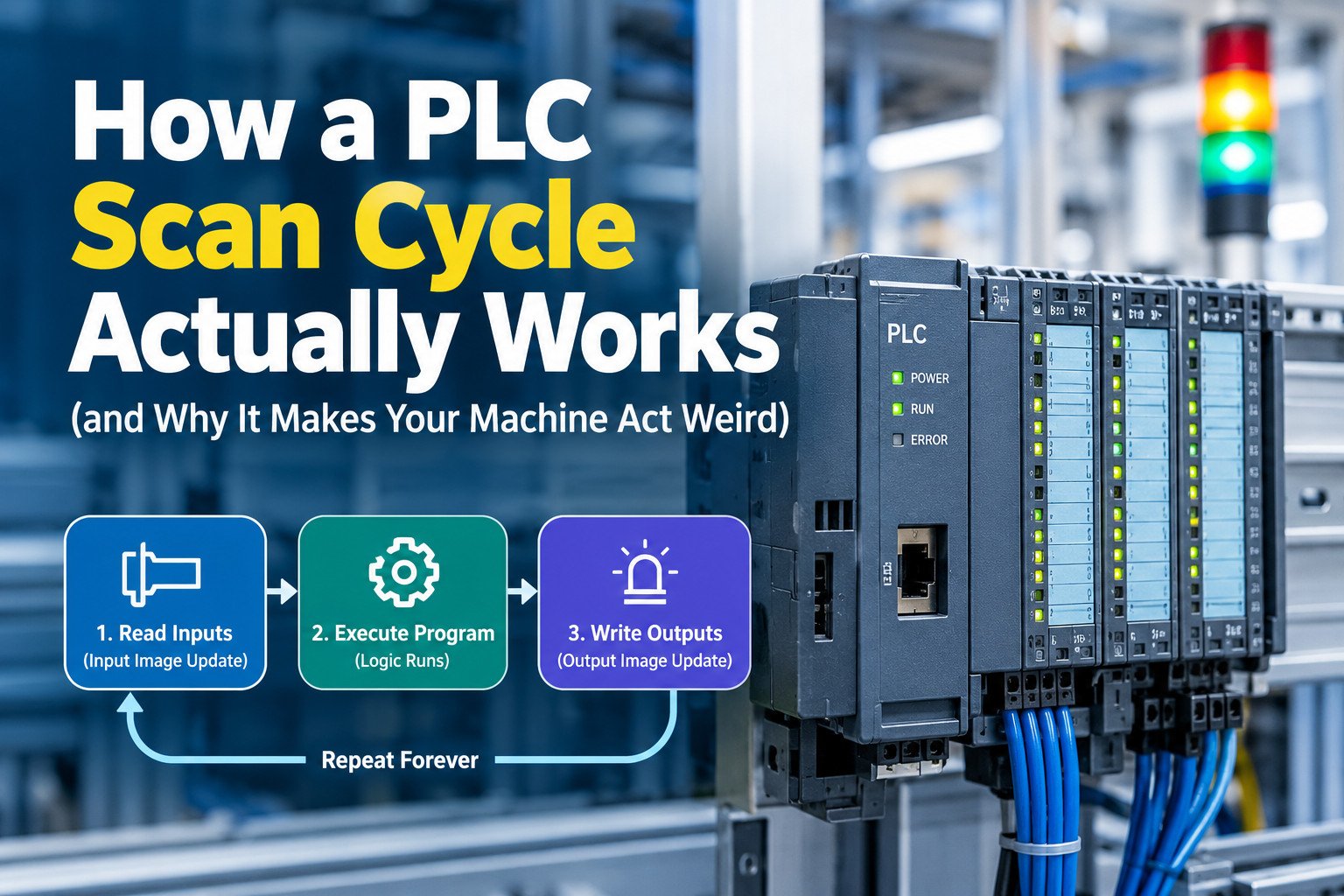
A programmable logic controller executes its user program in a repeating, fixed order. That order is called the scan cycle, and it is the single most important structural fact about any PLC. The specification for most controller families states this plainly, and every instruction reference manual assumes the reader understands it. When a machine behaves in a way that seems impossible – a sensor that fires but produces no action, a valve that opens a fraction of a second late, a fault that appears only at high throughput – the scan cycle is usually the explanation.
This article defines the mechanism precisely, in the sequence a controller executes it, and then connects that sequence to the symptoms maintenance technicians and machine builders actually report.
Quick answer: A PLC reads all its inputs into a memory copy, runs the entire program once using that frozen copy, then writes the results out. It repeats this forever. Anything that changes at a terminal while the program is running is invisible until the next pass.
What the scan cycle is and why the order matters
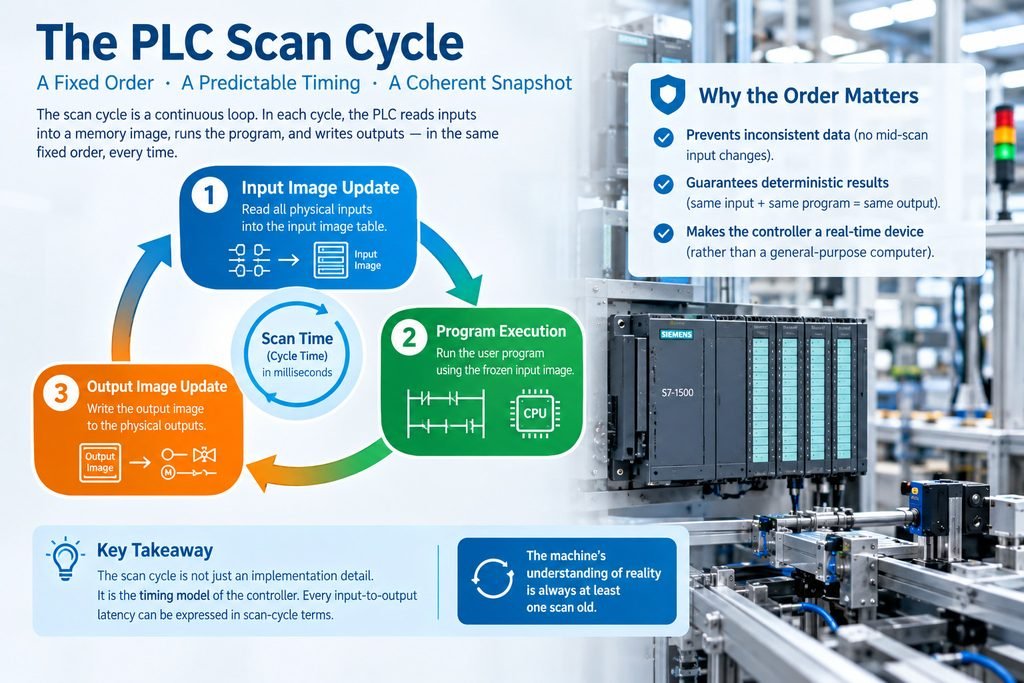
The scan cycle is a cyclic executive: a loop with no defined end, in which the controller performs the same set of operations in the same order, once per iteration. The duration of one iteration is the scan time, sometimes called the cycle time. The specification for most modern CPUs expresses this value in milliseconds and reports it as a running statistic.
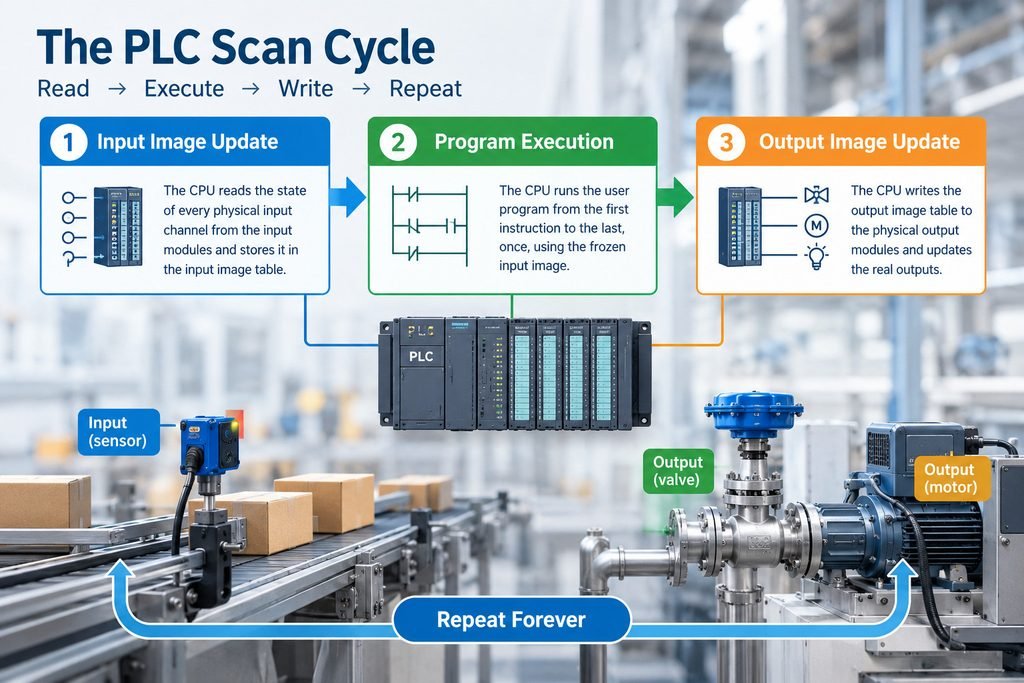
The order matters because of what the controller does not do. In the classic model, the user program never reads a physical input terminal and never drives a physical output terminal directly. Instead, the CPU maintains two dedicated blocks of internal memory: the input image and the output image. Each scan, the operating system copies the state of every physical input module into the input image, the program runs against that image, and then the operating system copies the output image out to the physical output modules.
This design exists for a specific reason: consistency. If the program could read terminals at arbitrary moments, a rung could evaluate input A as true, then evaluate input B a few microseconds later after B had already changed. The logic would act on a set of conditions that never existed simultaneously. By freezing every input into an image at one instant, the controller guarantees that one program pass sees one coherent snapshot of the machine.
The consequence is that the machine’s understanding of reality is always at least one scan old. An input that changes state immediately after the input image update will not be acted on. It will be acted on in the following scan.
Determinism follows from the fixed order. Given the same input image and the same program, the controller produces the same output image every time. The order of execution is defined by the program listing, not by the machine’s timing, not by interrupts from the field, and not by the speed of the processor at any given moment. This is what makes a PLC a real-time control device rather than a general-purpose computer.
A useful way to hold this: the scan cycle is not an implementation detail. It is the timing model of the controller. Every latency you measure on an input-to-output path can be decomposed into scan-cycle terms.
The three phases, in order
The classic model reduces the cycle to three phases. Real controllers execute more, but these three carry the logic.
Table 1: The three scan phases and what changes in each
| Order | Phase | What the CPU does | What is updated |
| 1 | Input image update | Reads the state of every physical input channel from the input modules | The input image table |
| 2 | Program execution | Runs the user program from the first instruction to the last, once | The output image table and internal memory |
| 3 | Output image update | Writes the output image table to the physical output modules | The physical output terminals |
Phase 1 is a sampling operation, not a subscription. The CPU reads each input channel’s current logical state and stores it. If an input turns on and off again between two samples, the controller records whatever state existed at the instant of each sample and nothing else. The intermediate activity is not queued.
Phase 2 executes the program. Rungs, function blocks, structured text statements, and sequential function chart steps all run in the order the programmer defined. The program may read the input image as many times as it likes and may modify the output image as many times as it likes. The only visible effect of those modifications within the same scan is on subsequent instructions reading the same tag.
Phase 3 transfers the output image to the output modules. After this transfer, the physical terminals reflect the logic that ran in phase 2.
A short trace makes the timing explicit:
SCAN N
t=0.0 ms INPUT IMAGE UPDATE –> image reflects part-present = OFF
t=1.2 ms PROGRAM RUNS –> program sees part-present = OFF
t=1.2 ms … (pulse arrives at terminal at t=4.0 ms)
t=8.4 ms OUTPUT IMAGE UPDATE –> outputs written from image
t=8.6 ms diagnostics / comms
SCAN N+1
t=20.0 ms INPUT IMAGE UPDATE –> image now reflects part-present = ON
t=21.2 ms PROGRAM RUNS –> program finally responds
t=28.4 ms OUTPUT IMAGE UPDATE
The input arrived at 4.0 ms into a 20 ms scan. The program did not learn about it until 20.0 ms, and the output terminal did not change until roughly 28.4 ms. That is the one-scan latency in concrete form.
Where the input image and the output image actually live
The input image and the output image are dedicated areas of the CPU’s memory system, separate from the physical I/O modules. On a modular system, the I/O modules sit on a backplane or a fieldbus; the images sit in the controller. The transfer between them is performed by the controller’s operating system, not by user logic.
Each scan, the CPU reads every configured input channel in the image, whether or not the program uses that channel. Each scan, it writes every configured output channel. The image size is therefore determined by the configured I/O, not by how much of the program is written.
This is the reason a program that references a dozen inputs still pays the cost of updating several hundred. Strictly speaking, the image update is proportional to the physical and configured channel count, and for a large remote I/O network carried on a fieldbus, the update also consumes communication bandwidth.
Two consequences are worth stating separately.
First, a program that writes to the same output coil in multiple places within one scan will leave the output in the state of the last write. The physical terminal never sees the intermediate states, because the transfer happens only in phase 3.
Second, a program that uses an immediate or direct I/O instruction – available on most platforms as a special instruction or a direct address form – temporarily bypasses the image. That instruction reads or writes the module at the moment it executes. It costs extra time and it breaks the coherence guarantee for that one access. Use it deliberately.
Warning: Immediate I/O instructions do not make the machine faster in general. They make one access current and everything else the same. Mixing them into logic carelessly produces the temporary conditions the image model exists to prevent.
Reading a real scan time
A real CPU cycle contains more than the three phases. A complete cycle typically includes internal diagnostics, communication and service processing, and operating-system time. Diagnostics verify memory integrity and module health. Communication processing handles programming-tool traffic, HMI requests, peer-to-peer messaging, and fieldbus service. Operating-system time covers scheduling, housekeeping, and the bookkeeping the controller performs for itself.
The datasheet scan time is a figure measured under a defined benchmark load, and it is not the whole cycle. The engineering manual will usually state the processing time per Boolean instruction and per word instruction, plus additional times for each I/O module and for each communication service. A realistic estimate combines those terms.
Table 2: Terms that make up a measured cycle on a real CPU
| Term | Origin | Typical share of a small program |
| Input image update | Configured input channels, local and remote | 5 to 20 percent |
| Program execution | Instruction count and instruction mix | 30 to 70 percent |
| Output image update | Configured output channels | 5 to 15 percent |
| Internal diagnostics | CPU and module supervision | 5 to 15 percent |
| Communication and service | HMI, programming tool, fieldbus, messaging | Variable, can dominate |
| Operating-system time | Scheduling and housekeeping | 5 to 20 percent |
The communication term is the one that surprises people. A controller with a light program and a heavily polled HMI, or one that is serving a large remote I/O ring, can spend more time on service processing than on logic. This is why the scan time reported immediately after a program download often climbs once the HMI and the network are connected.
Where the number is displayed, it is displayed as a statistic. On Siemens TIA Portal, the cycle time readout lives under Online and Diagnostics for the CPU, in the cycle time statistics view, which shows current, minimum, and maximum values. On Allen-Bradley controllers in Studio 5000, the task monitor shows task scan time, and the GSV instruction can be used to read task statistics into program tags so that the value is available to logic. On Mitsubishi GX Works3, the monitor view exposes the scan time of the running program. On Omron Sysmac Studio, the controller’s task execution time is available in the monitoring and troubleshooting views.
Siemens TIA Portal
Project tree > Devices > [CPU] > Online & Access
> Online & Diagnostics > Diagnostics > Cycle time
Observe: Current / Minimum / Maximum cycle time
Allen-Bradley Studio 5000
Controller Organizer > Tasks > [Task] > Monitor
Observe: Task Scan Time
In logic: GSV(Task, [TaskName], ScanTime, destination_tag)
Mitsubishi GX Works3
Online > Monitor > Scan Time / Program monitor
Omron Sysmac Studio
Controller > Monitoring > Task Execution Time
Read the maximum, not the average. The average scan time describes a machine that is behaving. The maximum scan time describes the worst pass the controller has performed, and that is the number that governs whether a short event can be missed.
Where the fixed order bites you
The classic field symptom of the image model is the missed pulse. Consider a machine that uses a photoelectric sensor to detect a part as it passes a station. The part is 40 mm long and travels at 1 m/s, so the sensor sees it for 40 ms. Now consider the same sensor on a machine running faster, where the part passes in 5 ms. If the controller’s scan time is 20 to 40 ms, the input image may never sample the sensor while the part is present.
The sensor is working. The wiring is correct. The input module’s indicator lights. The program never sees it.
Increasing CPU speed is the intuitive fix and it is usually the wrong one. To guarantee that a 5 ms event is always captured by sampling alone, the scan time would have to be well below 5 ms on every pass, including the worst-case pass, and it would have to remain below that value with margin for temperature and load. That is an expensive way to acquire a fact the hardware can acquire directly.
The correct fix is to move the detection out of the cyclic program and into hardware or into an interrupt. A high-speed counter input module counts pulses in dedicated hardware, independent of the scan. The program reads the accumulated count whenever it needs to, and no count is lost because the hardware never stopped counting. For logic that must respond to an event rather than to a sampled state, an interrupt routine is the appropriate mechanism: the event triggers the routine, which executes outside the normal cyclic order at a defined priority.
Most major platforms provide this. Siemens controllers support priority and cyclic interrupt organization blocks, which run at a configured priority and can interrupt the main cyclic program. Allen-Bradley controllers support event tasks and periodic tasks, which execute on a configured trigger rather than on the continuous task. Mitsubishi and Omron controllers provide interrupt execution and multi-program configurations in which a program or task runs at a defined priority or on a defined period.
These features solve the timing problem because they change where the logic runs, not how fast the CPU is. An interrupt routine runs when the event occurs. A high-speed counter counts when the pulse occurs.
Field note: A 5 ms part-present pulse on a machine with a 30 ms scan will be missed most of the time. The same pulse is captured reliably by a high-speed counter module, on the same CPU, with the same scan time. The CPU was never the limiting component.
Table 3: What a faster CPU does and does not solve
| Problem | Solved by a faster CPU | Solved by counters or interrupts |
| Short pulse missed by sampling | No, only by luck unless scan drops far below pulse width | Yes, by design |
| High-speed counting or position capture | No | Yes |
| Program too large to run in the required time | Yes, within limits | No |
| Slow HMI or messaging response | Partly | No |
| Deterministic response to an external event | No | Yes, via priority execution |
| Long scan caused by heavy communication | Partly | No, requires architecture change |
Scan time and response time are not the same number
Response time is the interval between a physical event and the resulting physical action elsewhere on the machine. Scan time is one term in that interval. Treating them as the same number causes most of the disagreement between a machine builder’s stated performance and a customer’s measurement.
The worst-case input-to-output delay in the simple local case is the sum of three delays: the input filter delay, the scan latency, and the output turn-on time. Most input modules apply a filter to reject noise, and that filter delays the appearance of a change at the module by its configured filter time. The scan latency is between one and two scan periods, depending on where in the cycle the event occurred. The output module has its own turn-on delay, plus the mechanical response of the device the output drives.
Table 4: One event, three different measured times on the same machine
| Measurement path | Delay terms | Approximate total |
| Local input to local output, event early in scan | Input filter 3 ms + scan latency 1 scan (20 ms) + output turn-on 2 ms | 25 ms |
| Local input to local output, event late in scan | Input filter 3 ms + scan latency 2 scans (40 ms) + output turn-on 2 ms | 45 ms |
| Sensor on a network input, action on a network drive | Network input delay + scan latency + network output delay + drive response | 50 to 120 ms |
The third row is the one that produces field disputes. When the sensor feeds a remote I/O block over a fieldbus and the output command travels to a drive over the same or another network, the network delays are added to the scan latency, and both networks have their own update periods. The same physical event that took 25 ms to propagate internally can take more than 100 ms end to end. The controller’s scan time is unchanged in both cases.
If your specification says the machine must react within a stated time, define where the clock starts and where it stops. Reaction time measured at the terminals of a local output is a different quantity from reaction time measured at the load, and both are different from reaction time measured through an HMI’s displayed status.
Bottom line: Scan time is a controller property. Response time is a system property. A machine can have a 10 ms scan and a 90 ms response time, and both numbers can be correct.
Tests you can run on your own machine
These procedures require only the controller, the programming software, and a way to change an input state. Run them before you accept a machine’s stated response time, and run them again after any program change that adds substantial logic or I/O.
- Record the cycle time statistics. Connect the programming tool, open the cycle time diagnostics view for the CPU, and let the machine run through a full production cycle. Note the current, minimum, and maximum values. The maximum is the figure you will use in all subsequent calculations.
- Record the actual maximum under load. Repeat the recording while the HMI is displaying an active screen, while messaging is enabled, and while any other network clients are connected. Controller scan time commonly rises when service processing is present.
- Measure one input-to-output delay with an oscilloscope or a high-resolution logging tool. Connect one channel to the input terminal and a second channel to the output terminal. Trigger on the input edge. The interval between edges is the real delay for that event, on that path, in that scan position.
- Repeat the measurement at least twenty times. The delay will vary by roughly one scan period because the event lands in a different position in the cycle each time. The spread confirms the mechanism.
- Test the missed-pulse case deliberately. Generate a pulse of known width at an input and log whether the program registers it. Vary the pulse width from well above the scan time down to a fraction of it. The pulse disappears from the program’s view at the width where sampling can no longer catch it.
- Replace the input with a high-speed counter channel and repeat step 5. The count should be captured at pulse widths far below the scan time.
- Log the counting behavior under maximum load. Confirm that the counter still captures pulses while the scan time is at its maximum.
Use this checklist to keep the measurements repeatable:
☐ Cycle time statistics recorded with current, minimum, and maximum values
☐ Maximum scan time recorded with HMI, messaging, and network clients active
☐ Input-to-output delay measured at the terminals, not from a screen
☐ Measurement repeated at least twenty times to establish the spread
☐ Pulse-width threshold established where the program stops seeing the event
☐ Counter or interrupt input verified at widths below the scan time
☐ Filter times read from the input module documentation for each channel
☐ Output turn-on time read from the output module documentation
☐ Network update periods recorded for any remote I/O or drive path
☐ All recorded values compared against the machine’s stated response requirement
Keep the recorded values with the machine documentation. When a customer later reports a timing complaint, the numbers answer the question before anyone opens the panel.
Rules of thumb for sizing a CPU against a scan time
Sizing decisions are easier when the expected scan time is estimated before hardware is purchased. The table below gives typical ranges for well-written programs on each controller class. These are ranges from practice, not guarantees, and they shift with I/O count, program size, and communication load.
Table 5: Typical scan time ranges by controller class
| Controller class | Typical scan time | Typical application |
| Brick or micro PLC | 1 to 10 ms | Standalone machines, small enclosures, simple sequencing |
| Compact modular PLC | 5 to 25 ms | Multi-station machines, moderate I/O counts, HMI and small networks |
| Large modular or process controller | 20 to 100 ms | Process control, large remote I/O, many loops and analog channels |
A 10 ms scan is generally more than adequate for a conveyor, a tank level loop, a temperature control loop, or a sequence of valve and motor steps. Human perception and mechanical response in those applications operate on much longer scales. A 10 ms scan is hopeless for a registration mark, an encoder edge, a flying cut, or any event whose duration is comparable to the scan itself. Those applications need dedicated hardware or interrupt-driven execution regardless of the CPU class.
Size for the maximum, not the average. Add the estimated program time, the image update time for the configured I/O, and an allowance for communication. Then compare that figure against the shortest event the machine must reliably detect. If the shortest event is less than several times the maximum scan time, the design needs a counter input, an interrupt routine, or both. If the shortest event is comfortably longer than the maximum scan time, the cyclic model is sufficient and a faster CPU buys nothing that the application needs.
The design rule that follows from this is simple. If the event you must detect is shorter than a few scan periods, do not design around the scan. Design around hardware that runs independently of it.
Watchdog supervision closes the loop on scan-time management. Most controllers allow a maximum scan time to be configured, and the operating system monitors the actual scan against that limit. If the program exceeds the limit, the CPU raises a cycle-time or watchdog fault and normally transitions to a safe state, which usually means de-energizing outputs according to the configured behavior.
The usual causes of a scan-time fault are predictable and are worth checking in this order.
- Nested loops over large arrays, where the instruction count grows with the product of the loop bounds.
- Large iteration counts in loop constructs, where a single instruction block repeats thousands of times in one pass.
- An excessive number of configured I/O channels in the image, which inflates the update time even when the channels are unused.
- Slow or blocking block reads, including reads from memory cards, file operations, or non-optimized data access.
- Communication calls placed in the main cyclic program, where a wait for a network reply stalls the whole scan.
- A one-time diagnostic routine, startup sequence, or data conversion that runs in the main task instead of in a separate or triggered task.
The remedy is almost always structural. Move heavy loops into a lower-priority or triggered task, move communication calls out of the main cycle, reduce the configured I/O to what the machine actually has, or split a large program across tasks so that the time-critical logic executes every scan while the bulk logic executes less often.
Two related questions come up often enough to answer here. First, whether an older controller can be made faster by rewriting the program: within limits, yes, because instruction count is the dominant term for most programs, but the floor is set by the image update and the operating-system overhead. Second, whether a faster controller removes the need to think about timing: no, because the missed-pulse problem is structural rather than computational, and a faster CPU simply moves the threshold at which it appears.
For readers assembling or replacing hardware, the available control and monitoring hardware is worth reviewing alongside the controller’s documented scan time figures, since the input module’s filter time and the output module’s turn-on time appear in the total delay.
If you are new to the device itself, the plain-language explanation of what a programmable logic controller does provides the background this article assumes, and further technical notes are collected in the news and technical articles section.
When the machine and the program both behave correctly and the timing is still wrong, the scan cycle is the explanation more often than any other single mechanism. The controller is not slow. It is ordered.